Logistic Regression: A Guide to Understanding the Basics

Logistic Regression – a concept that sounds somewhat academic, yet it’s used every day in various fields including machine learning. But fear not! This article is here to unmask this seemingly complex subject and make it accessible to everyone, even those without a PhD in statistics. Let’s take a step-by-step look at what Logistic Regression is, why it’s important, and how to get started using it.

Introduction

Logistic Regression is not as daunting as it sounds. It’s a statistical model used for binary classification. In simpler terms, it helps in predicting a binary outcome (1 / 0, Yes / No, True / False) given a set of independent variables.

Independent Variables

Independent variables, also referred to as predictors or features, are the variables that are manipulated or categorized to observe their effect on dependent variables. In the context of Logistic Regression, these are the variables that are used to predict the outcome.

Example: In predicting whether a particular email is spam or not, the independent variables might include the frequency of certain words in the email, the sender’s email address, the time it was sent, etc.

Dependent Variables

Dependent variables, also known as the response or target variables, are the outcomes we’re interested in predicting or explaining. They depend on the values of the independent variables.

In Logistic Regression, the dependent variable is usually binary, meaning it has only two possible outcomes.

Example: Continuing with the email spam example, the dependent variable would be a binary classification: ‘spam’ or ‘not spam’.

The relationship between independent and dependent variables can be expressed mathematically in the form of a function. In the context of Logistic Regression, the dependent variable is modeled using the Sigmoid function, where the independent variables are inputs to predict the probability of a particular class.

Introduction to Classification Problems

In the world of machine learning, a multitude of problems are awaiting robust solutions. One of the most central and widely tackled problems is that of classification. But what exactly is a classification problem?

A classification problem is essentially a type of puzzle. Imagine you have a basket filled with fruits, and you want to sort them into different baskets labeled as ‘Apples’, ‘Oranges’, ‘Bananas’, and so forth. This sorting, or categorizing, is what classification is all about.

In the context of machine learning, classification problems are all about categorizing or labeling data points into specific classes or groups. It’s like teaching a computer to sort the fruits for you!

Binary and Multiclass Classification

Classification problems can be broadly divided into two categories:

Binary Classification: This involves categorizing the data points into one of two possible classes. It’s a yes-or-no, true-or-false type of decision-making process. For example, determining whether an email is spam or not spam.
Multiclass Classification: This is a bit more complex, involving more than two classes. It’s akin to sorting those various types of fruits. In the world of data, it might involve categorizing news articles into different genres like politics, sports, technology, etc.

Why Logistic Regression?

Now, where does Logistic Regression fit into this classification landscape?

Logistic Regression is a powerful yet elegant statistical method used to solve binary classification problems. It’s like a wise guide helping you navigate the complex terrain of data, finding the right path to categorize each piece of information accurately.

The beauty of Logistic Regression lies in its simplicity and effectiveness. Using the mathematical function called the Sigmoid, Logistic Regression calculates the probability that a given data point belongs to a particular class. If the probability is above a certain threshold, the data point is labeled as belonging to that class.

Logistic Regression can also be extended to solve multiclass problems, making it a versatile tool in the machine learning toolkit.

In a Nutshell

Classification is a fundamental task in machine learning, and Logistic Regression is one of the go-to methods to solve binary classification problems. Whether it’s categorizing emails as spam or not, detecting fraudulent transactions, or any other binary decision-making task, Logistic Regression is often on the front lines, providing reliable and interpretable results.

Linear vs Logistic Regression

Understanding the difference between linear and logistic regression is vital. Let’s break it down:

Linear Regression:
- Predicts continuous outcomes.
- Often visualized as a straight line.
Logistic Regression:
- Predicts binary outcomes.
- Uses a logistic function to model a binary dependent variable.

Note: Though they share the name “regression,” their applications are quite distinct.

Comparison with Linear Regression

Logistic Regression and Linear Regression are often mentioned in the same breath, but they are designed to address different types of problems. Though their names might sound similar, and they share some fundamental concepts, the differences between them are profound. Let’s explore these differences side-by-side.

1. Objective

Linear Regression: It is used to predict a continuous value. For instance, predicting house prices based on various features like size, location, etc.
Logistic Regression: It is used for classification, specifically binary classification. It predicts the probability that a given instance belongs to a particular class.

2. Output

Linear Regression: The output is a real number, representing a point on a continuous scale.
Logistic Regression: The output is a probability value between 0 and 1. It’s then mapped to a discrete class label.

3. Function Used

Linear Regression: Employs a linear function to fit the data.
Logistic Regression: Uses the logistic (or Sigmoid) function to squeeze the output between 0 and 1, thus aiding in classification.

4. Loss Function

Linear Regression: Utilizes Mean Squared Error (MSE) to calculate the difference between the predicted and actual values.
Logistic Regression: Relies on Log Loss, which measures the performance of a classification model where the prediction input is a probability value between 0 and 1.

5. Assumptions

Linear Regression: Assumes a linear relationship between the input features and the output.
Logistic Regression: Does not assume a linear relationship between the input features and the output but assumes linearity between the input features and the log-odds of the output.

6. Usage Scenario

Linear Regression: When you need to predict a quantitative response.
Logistic Regression: When the task at hand is a classification, especially binary classification.

Why Logistic Regression for Classification?

Linear Regression could theoretically be used for classification, but it’s not suited for the job. Here’s why Logistic Regression shines for classification tasks:

Probability Estimation: Logistic Regression doesn’t just classify; it provides a probability score underpinning the classification. This information can be valuable in understanding the confidence of the model in its predictions.
Threshold Tuning: By adjusting the decision threshold, you can tune the model to be more sensitive or specific, depending on the problem’s requirements.
Robust to Noise: It’s more robust to noise and can handle data points that don’t strictly follow the linear assumption.

In Summary

While both Logistic and Linear Regression are essential tools in machine learning, they are applied to distinct types of problems. Logistic Regression’s design makes it a natural fit for classification problems, whereas Linear Regression is tailored for regression tasks.

The choice between Logistic and Linear Regression is not just a matter of preference but of applying the right tool for the right job. In the world of binary classification, Logistic Regression is often the wise choice, thanks to its ability to provide probability estimates and its robustness in handling real-world data quirks.

The Sigmoid Function

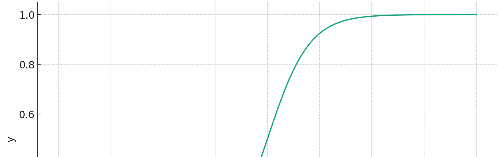
In Logistic Regression, we use something called the Sigmoid function. It’s a fascinating curve that transforms any value into a number between 0 and 1, making it perfect for probability estimation.

Here’s the mathematical expression:

S(x)=1+e−x1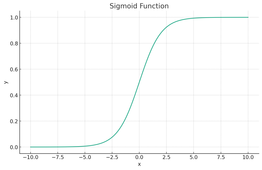

It may look complex, but the beauty of this curve is in its simplicity. As x approaches infinity, the value of S(x) nears 1, and as x approaches negative infinity, S(x) nears 0. This characteristic ensures that our predictions remain within the range of 0 and 1.

Cost Function

The Cost Function is at the heart of Logistic Regression. It’s the measure of how well the algorithm is performing. A lower cost means better performance, and our goal is to minimize this cost.

Here’s the cost function for Logistic Regression:

math

J(θ) = - (1/m) * ∑ [y log(hθ(x)) + (1 - y) log(1 - hθ(x))]

m is the number of observations.
y is the actual value.
hθ(x) is the predicted value.

Confused? Don’t be. It essentially calculates the difference between the actual and predicted values. This function might appear abstract, but it plays a crucial role in training the model.

Gradient Descent

Gradient Descent is the method used to find the minimum of the cost function. It’s like navigating a mountainous terrain to find the lowest valley.

Here’s a simplified explanation:

Start at a Random Point: Choose an initial set of parameters.
Calculate the Gradient: Determine the slope of the cost function at the current point.
Update the Parameters: Move in the opposite direction of the gradient. The size of each step is determined by the learning rate.
Repeat Steps 2 and 3: Continue until the slope is near zero, indicating that the minimum has been reached.

In mathematical terms:

θj = θj - α * ∂/∂θj * J(θ)

θj is the parameter being updated.
α is the learning rate.
∂/∂θj * J(θ) is the gradient of the cost function.

A Simple Python Tutorial

Now, let’s roll up our sleeves and dive into some coding. We’ll use the widely available IRIS dataset.

Step 1: Importing Libraries

import numpy as np
from sklearn.datasets import load_iris
from sklearn.linear_model import LogisticRegression

Step 2: Loading the IRIS Dataset

iris = load_iris()
X = iris.data[:, (2, 3)] # Using petal length and width
y = (iris.target == 2).astype(int) # We'll predict if it's a specific species

Step 3: Creating and Training the Model

model = LogisticRegression()
model.fit(X, y)

Step 4: Making Predictions

test_data = [[5.1, 2.4]]
prediction = model.predict(test_data)
print(f'Prediction: {prediction}')

This simple code snippet can predict whether a given iris flower belongs to a specific species based on its petal length and width.

Conclusion

In this journey through Logistic Regression, we’ve unraveled the mathematical essence, the elegance of the Sigmoid function, and even got our hands dirty with some Python coding. As an integral part of machine learning, understanding Logistic Regression is like possessing a key to a treasure trove of predictive analytics.